There’s a famous story about Richard Feynman at Cornell suffering from the science equivalent of writer’s block, after WWII. He was depressed and feeling like everything he did was pointless, until one day he spotted a student throwing a plate up in the air in the cafeteria. As the plate spun, it wobbled, and the wobble seemed to go faster than the spin. Intrigued, he sat down and calculated the physics involved, finding that, indeed, the wobble should go at twice the rate of spin. This basically reignited his interest in physics, and shortly after that, began his legendarily productive period when he invented his version of QED.
I mention this not to put myself in Feynman’s category, but just as a reminder of the universal tenddency of physicists to get caught up in looking at silly, simple problems in more detail than is really required. Such as, for example, the several hours I spent this week simulating the motion of a pendulum in VPython.
Like a lot of things these days, this came out of a passing mention on Twitter: Andrew Morrison was asking about using a pendulum in a lab as a demonstration of conservation of energy, and I got brought into the conversation. This, in turn, got me thinking about simulating a pendulum, something I’ve wondered about in the past, particularly when I was doing a seminar on timekeeping.
I had toyed with the idea of using a simulation to demonstrate the physics of a pendulum, and how its period depends on the angle, as this is a big issue for making accurate pendulum-based clocks. If you use a really wide swing for a pendulum, it takes longer to complete an oscillation than you would expect from a simple model. You can calculate approximately how much it varies, but the math is kind of hairy, and a simulation is probably more engaging, anyway.
I ended up not doing it because when I started thinking about it, the obvious way to do it was to just stick in the necessary force, which I can easily calculate– the “string” of the pendulum needs to pull on the bob with a force equal to to outward component of gravity plus the centripetal force needed to keep it on the right arc. The problem is, that seems like a cheat– I’ve calculated the force needed before doing the simulation, which defeats the purpose of the simulation, and brings in a bunch of physics that goes beyond what I wanted to deal with.
As usual, I was being an idiot, and when the Twitter conversation got me thinking about this again, I realized that the Matter and Interactions textbook that got me into simulating things in VPython in the first place also provides an explanation for how to calculate the motion of a pendulum without putting the force in by hand. The book spends a whole bunch of time on a microscopic model of material objects as balls (atoms) connected by springs (chemical bonds). So, the solution is simple: treat the string of the simulated pendulum as a spring. The idealized version of a pendulum, after all, that provides whatever force it needs to to keep the ball on a set path, is just a spring with an infinite spring constant, giving a finite force for an infinitesimal stretch.
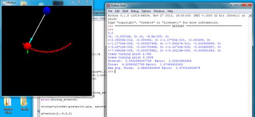
Once you do that, it’s easy to code up, and doesn’t require any prior knowledge of the path. Of course, you need some idea of what to use for a spring constant, but then the beauty of this method is that you can just stick in any value you like, and see what happens. The screen shot at the top is for a spring constant of 100 N/m (not all that strong) and a starting angle of 37 degrees (which is close to the small angle of a 3-4-5 triangle). The program assumes the spring-string is at its relaxed length to start, so providing no force, and the red trace in that image shows the resulting path, which makes a cool pattern.
That motion can be broken down into two pieces: there’s a mass-on-a-spring oscillation in and out, as the spring-string stretches and compresses; the period of that is pretty much exactly what you expect for the spring constant and mass in the simulation. Then there’s the back-and-forth oscillation of the pendulum on a mostly circular arc. For this particular choice of parameters, these periods are close to commensurate, so the pendulum more or less retraces its own path, giving a nifty pattern. For a different choice of angle, the path sort of smears out into a broad band after several oscillations.
Of course, the interesting thing to do with this is to look at how the period depends on angle, as I toyed with doing back when I taught about timekeeping. Measuring the period for a bunch of different angles gives the following graph:

The red points here represent the simulation for a spring constant of 100 N/m, as in the above screen shot. You can see that, as you expect, the period increases slightly as you go to larger angles. The theoretical value for an ideal pendulum is 2.0071s, and all of these points are higher than that, presumably because the stretching of the pendulum increases the effective length as it swings.
There are three other sets plotted here, as well, though it’s hard to see them. There are black circles, labeled “cheat” for the simulation where I put in the formula for the right force by hand. These are almost impossible to see, because they’re under the yellow triangles from the simulation for a spring constant of 10,000 N/m; almost all of these are within 0.0001s of the “cheat” values. There are also green triangles, for a spring constant of 1,000 N/m (half as many, because I got tired of copying down values), which are very slightly higher than the 10,000 N/m points, but not by all that much.
So, this does exactly what you would expect: as you increase the spring constant, the period value approaches the “ideal” case of a string that doesn’t stretch at all. Physics works, hooray!
It’s sort of interesting to look at how that approach happens, so here’s another graph:

This shows the period for a single starting angle– 37 degrees– for a bunch of different spring constants. Note that the horizontal scale is logarithmic, so this spans a range from 10 N/m to 100,000 N/m. The dashed horizontal line is the “cheat” value of 2.0610s. This is a few hundredths of a percent from the approximate theoretical value for that angle, so again: physics works, hooray! I don’t have a particular expectation for what the approach to the ideal value should look like, mathematically, or I’d fit a function to those points. This looks pretty reasonable, though.
So, the upshot here is that it is, in fact, possible to simulate the motion of a simple pendulum very well without knowing the right answer in advance. This also produces a slightly surprising result, namely that the force on the string oscillates rapidly during the whole swing, as the spring-string stretches and compresses. At any given instant, the force can be substantially less or substantially more than the theoretical value for the “cheat” version. This isn’t something you’d necessarily anticipate, but it does make sense when you think about the underlying physics. I didn’t make graphs of this, but did look at the ratio of the maximum force measured through the swing and the “theoretical” maximum that you expect from the “cheat” model. These numbers were very consistent across the different spring constants, and varied with the angle in a kind of interesting way: the larger the starting angle, the smaller the ratio of the two.
Again, this makes some sense if you think about the underlying physics: the initial condition of the model is that the spring-string is unstretched, and thus exerting zero force at the starting point. This is a good fit at large angles– the “cheat” model would give zero force for an angle of 90 degrees. At smaller angles, though, this is a very bad approximation, so you would expect the simulation to deviate from the ideal by a larger amount. At 85 degrees, the maximum force is about 3% more than the “cheat” version, while at 5 degrees it’s close to a factor of two larger.
You can also do a time-average of the force over one of the radial oscillations (basically adding up the force for each time step between reversals of the velocity along the string, then dividing by the number of time steps), and look at that. As you might well expect, this tracks the “cheat” value reasonably well, coming within a few percent for most of the oscillation. It tends to come in a little low, which might just be a numerical artifact due to the fact that I’m a lousy programmer.
The obvious extension of this is to correct the zero-force assumption at the starting point– in reality, if you start a pendulum, you stretch the spring so it’s under a slight tension, so the string is taut. In principle, I think there should be a position where the spring-string ought to smoothly stretch to always be exactly the length it needs to be to supply the necessary centripetal force. It’s not obvious how to calculate the right starting position, though, and I’ve spent enough time futzing around with this is it is, so let’s just leave that as a homework exercise for the interested reader. (If I get bored enough in the near future, I may try to trial-and-error my way to the right value…)
So, anyway, there’s the latest in my open-ended series of overthinking the physics of simple systems. I’m not sure this will actually be any use in a class, unless I end up teaching our intermediate mechanics course– the issues involved in this end up going well beyond the content of our introductory courses (even though it was Matter and Interactions that kicked the whole thing off…). But it was fun to work up, and good enough for a blog post…
Relaxing a rigid body constraint by using springs is a pretty common technique, and it’s also used in static problems. Typically if you have a statically indeterminate situation, like finding the force in the legs of a four-legged table, you HAVE to relax the problem or you can’t solve it. (One dimensional equivalent: five people carry a log, how much is each person lifting if they carry the log at the same height?)
* re “force in the legs” — I mean the force of the legs on the floor.
As I said, once I realized what to do, I felt like an idiot. The spring approach is obviously the way to go.
I forgot to mention, though, that my initial attempts to increase the spring constant kept running into numerical issues, because of course, when the radial oscillation frequency gets too high, you start having issues with overshoot, and then the force gets gigantic.
First I must say I’m no physicist but it was one of my best subjects in college. In your approach to the pendulum problem you’re thorough and adequate for practical purposes but there’s much more to the problem than meets the eye. To really get down to the nitty-gritty and get real precision in your solution you need to account for things like the variability of gravity depending on your position on Earth and air resistance depending on the shape of the pendulum and the friction of the pendulum’s fulcrum. All of these effects are very small, of course, and can be neglected in most cases. I just think it’s important to be aware of them so you can decide whether to use them.
Overall, this was a neat project and well handled.
Wouldn’t the natural thing to do would be to add damping to the spring? That should reduce the oscillation problem.
Damping the spring and adding air resistance are obvious future steps, yes. The damping would be even more ad hoc than the spring constant, though; I have a very rough sense of what order of magnitude to put on the spring constant (Matter and Interactions does a bunch of stuff with the effective spring constants of metal wires, which generally come out on the order of 100,000 N/m, so a string should be less than that), but I have no clue regarding damping. Air resistance, there’s an empirical formula for, at least.
Also, I probably should’ve included the code for this simulation, but it’s kind of illegible crap, and putting in comments to make it make sense would take forever…
The thing I found most interesting about combining a pendulum with a spring is the fact that there exists a chaotic configuration. If one chooses the mass so that the spring is elongated by IIRC 3/4 of its base length, then it becomes impossible to get anything even remotely periodical. We calculated this thing in 3rd semester physics, and the professor called it an ‘auto-parametric oscillator’, but I never found it in the literature.
Hate to nitpick, but the spin was 2x the wobble (for small values of wobble), not the other way around. “I noticed the red medallion of Cornell on the plate going around. It was pretty obvious to me that the medallion went around faster than the wobbling.”
I remember this because a spinning plate is almost too fast to track – only the medallion let him do it…. the wobble had to be slower or he wouldn’t have seen it.
I now wonder if he subconsciously picked up on the 2:1 sync – I don’t remember if he’d taken up bongos at that point.
Memo to self: must keep eyes open and brain turned on.
Update: Oh, hell. Feynman misremembered – the wobble is faster than the spin… Prof. Orzel is (of course) correct. 🙁
So how the hell did Feynman spot the spin vs. blur?
@Lurker: Wobble should be easier to see than spin, at least if the magnitude of the wobble is large enough. To detect spin you have to be able to track the motion of some fiducial mark, which in Feynman’s case was the Cornell logo. Wobble means that the orientation of the plate is changing; instead of focusing on a single point, you are watching what happens to the entire plate. It’s as if you are tracking the envelope of how a single point might move, rather than how a single point actually moves. The frequency at which this motion becomes a blur will be much higher for most people than the frequency at which the spin becomes a blur.
@Eric: I’ve just tried doing the experiment with an old driver CD, and I can see the wobble and the spin – but short of bouncing it off the ceiling, it’s not in the air long enough to get much of an impression. (Friday afternoon = throw my own damn CDs).
Odd that nobody has a good demo of this on Youtube.
Clearly, you need to lurk in a place with a higher ceiling…
Maybe I’ll try this with a frisbee later.
3m not enough…. It’s the rapid change in viewing angle that makes it hard. A larger target at a greater distance, rotating more slowly is probably a better way to go about it.
Of course, a very horizontal spinning axle through the CD’s hole (axle diam < CD hole diam) would allow for a stationary video. Spin it up a bit and perturb it gently. The CD's reflective surface is very good for seeing the wobble, and some ink dots for seeing the rotation. It's the parabola-at-close-range that's the problem…. 🙁
Springy pendulums have all sorts of cool physics ideas imbedded in them (e.g., Hamiltonian monodromy). My group got really into them a few years ago. We even got a paper published in PRL where the experimental apparatus was just a mass on a spring, which I thought was pretty cool.
http://physics.aps.org/synopsis-for/10.1103/PhysRevLett.103.034301
Damping as a whole is pretty ad-hoc, as I understand it. You just try several coefficient values until you find something that matches experimental results.
Air resistance is Reynold’s number dependent, so perhaps you should model the switching from Stokes flow to mid-Reynold’s number. You know, just to make things fun.
Have I noticed a tenddency for physicists to spell tenddency with two dd’s? or is it an anomaly?
Does the word ‘tend’ invoke a bias towards repetition?